Winter Solar Power is a Two-Humped Camel: Math Really Works
The graph below shows Nevada’s utility-scale solar generation by hour of the day, for each month. This post uses math (trigonometry and linear algebra) of solar angles and the physical attributes of utility-scale solar panels to explain the funny shape of the curves.
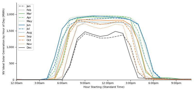
Two features are notable:
-
Long hours of consistently high output in summer rather than a sharper midday crest. Of the roughly 14 hours per day of production in June, 10 of those are at least 90% of the peak: the intensity drops off only during the two hours after sunrise and two hours before sunset.
-
The “dip” in mid-day in winter months. The best solar generation does not occur when the sun is highest in the sky at mid-day, but in peaks before and after.
As we’ll see, the data is consistent with single-axis solar tracking panels adjusts the position of a solar panel along one axis of rotation (i.e., east to west) to make the sun’s rays strike the panel as close to perpendicular as possible. By pointing east in the morning, rotating to be horizontal at mid-day, and then pointing towards the west in the afternoon, a tracking panel can lengthen the period of time that the sun’s rays strike at a near-perpendicular angle to the panel.
In the winter, the two-humped shape occurs because the sun is overall quite low in the sky. In the mid-day the sun is in the south. The best the panel can do is to be horizontal, but the sun is so low that the angle of incidence is far from perpendicular. Better angles – and more electricity generation – occur in the morning and afternoon when the sun is further east or west. This dip does not occur in the summer because the sun is high enough in the sky that a horizontal panel still has a close-to-perpendicular angle at midday.
The strong hours in the summer are particularly long because the sun rises in the north-east, and gets to due east around 9:00 a.m. (8 a.m. standard time). At this point an east-west orientation can point a panel directly at the sun. Ih the afternoon, the sun gets to due west around 5:00 p.m. (4 p.m. standard time). So the hours where the panel can get a nearly-perpendicular angle to the sun span more than this 8-hour period.
There are more subtle features of the generation chart that are less intuitive. First, the maximum generation generation months do not appear to be symmetrical around June (the month with the most daylight hours), but instead appear skewed towards the spring: April and May see more solar generation than July and August. It’s not obvious why this would be the case. In addition, the darkest winter months of December / January seem to be particularly low-generation outliers (i.e., November and February represent big steps-up in generation).
This post, by deploying a simple conceptual model of the physics and math of solar panels, explains these phenomena. Let’s dig in.
A Simplified Model of Solar Panels
I don’t have enough information (e.g., number of panels deployed) to estimate the absolute power output of utility solar generation in Nevada. However, by using basic information about the angle of the sun, the likely position of panels, and data about the intensity of the sun’s rays, we can generate an estimate of the output of solar panels relative to their maximum output, and so can validate the shape of the generation curves above.
The collection of solar radiation by a PV panel is on the flux of solar energy through the surface: sunlight shining perpendicular to the panel geneartes the most energy; sunlight parallel to the surface generates no energy; for any angle it’s the component portion of the sunlight that is perpendicular to the panel that we’re looking for.
Hence we want to measure the angle between that vector and the normal (perpendicular) vector \(\vec{N}\) to the panel’s surface. If those vectors have zero angle between them, the sun is shining perpendicular to surface, and energy is maximized. Higher angle means the sun is shining less directly on the panel. Mathematically, the solar energy that the panel can capture is proportional to the cosine of the angle between the sun’s position vector and the normal vector of the solar panel.
Sun Position
Imagine our solar panel is at the origin in a 3-dimensional plot. The vector of sun’s position is described with two angles.
- The elevation angle of the sun above the horizon, which I denote as \(\phi\) (this can go from 0° at the horizon to 90° directly overhead)
- The azimuth angle, which is the direction on the horizon that the sun is over, ranging over 0° for North, to 90° East, 180° South, 270° West and up to 360° to go back to North.
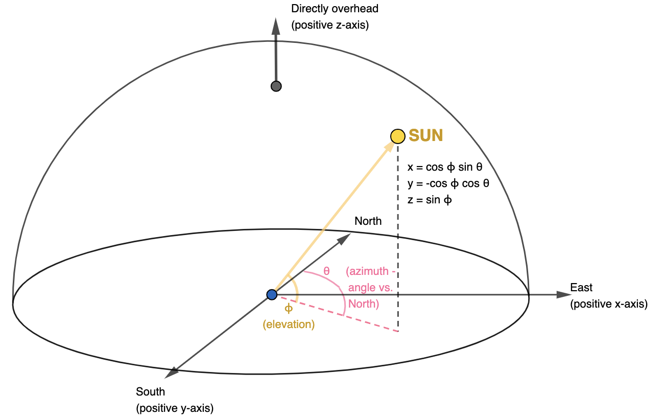
We’ll eventually want to find the angle between the sun’s position vector and the vector normal to a solar panel on the ground, so we’ll derive the (x, y, z) coordinates of the sun’s position on a unit sphere from the angles. From triangle trigonometry, the z-coordinate is simply 1 times the sine of the elevation angle, \(sin\ \phi\). Similarly, the length of the distance from the origin to the projection of the sun onto the xy plane is \(cos\ \phi\). The x and y coordinates are then the projections of that point onto the x and y axis using the azimuth angle: the x-coordinate is \(cos \phi\ sin \theta\) and the y-coordinate is \(-cos \phi\ cos \theta\) (the negative sign comes from my chosen orientation of the positive y-axis as being south). Thus the position vector of the sun ends up as the unit vector \([cos \phi\ sin \theta,\ -cos \phi\ cos \theta,\ sin \phi]\).
Finding these two angles for the sun’s position at any location on Earth at any time is a straightforward computation based on longitude, latitude, time of day and day of year (and timezone).
Here’s a few examples:
| 8:00 a.m. | 10:00 a.m. | 12:00 noon | 2:00 p.m. | 4:00 p.m. | ||
|---|---|---|---|---|---|---|
| June 15 | Elevation | 41.1° | 64.8° | 76.5° | 57.4° | 33.3° |
| Azimuth | 89.3° | 113.7° | 199.3° | 256.5° | 276.1° | |
| September 15 | Elevation | 30.5° | 50.3° | 56.5° | 43.1° | 21.0° |
| Azimuth | 110.5° | 140.6° | 191.0° | 233.7° | 257.9° | |
| December 15 | Elevation | 11.8° | 26.4° | 30.3° | 21.5° | 3.9° |
| Azimuth | 130.6° | 155.4° | 186.4° | 215.5° | 237.3° | |
Notice that in June, the sun spends more than 8 hours at an angle higher than the maximum elevation of the sun in December.
Single-Axis Tracking Panels
For a single panel, solar yield is maximized by dual-axis tracking: which can be rotated on two axes (e.g., horizontal and vertical) to point at any point in the sky. But most utility scale solar arrays (including those in Nevada) are single-axis trackers, and look like the below near Las Vegas:
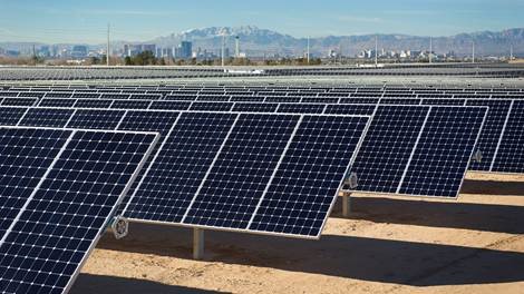
The panels sit in long parallel rows and can be most efficiently managed and spaced by rotating them together on a single axis of rotation (i.e. rotating a single bar rotates the entire row of panels). Here, a horizontal axis that allows the panels to point east in the morning, tilt towards horizontal to point overhead at mid-day, then point towards the west in the evening, will be optimal.
Finding the Angle of Incidence and then Optimizing It
Imagine that we tilt our solar panel an angle \(\alpha\) away from vertical, with positive \(\alpha\)’s toward the east and negative \(\alpha\)’s toward the west. Again assuming a unit sphere model of the sky, the east-west orientation means that the direction the panel points lies on the xz plane, at the unit vector \([sin\ \alpha, 0, cos\ \alpha]\).
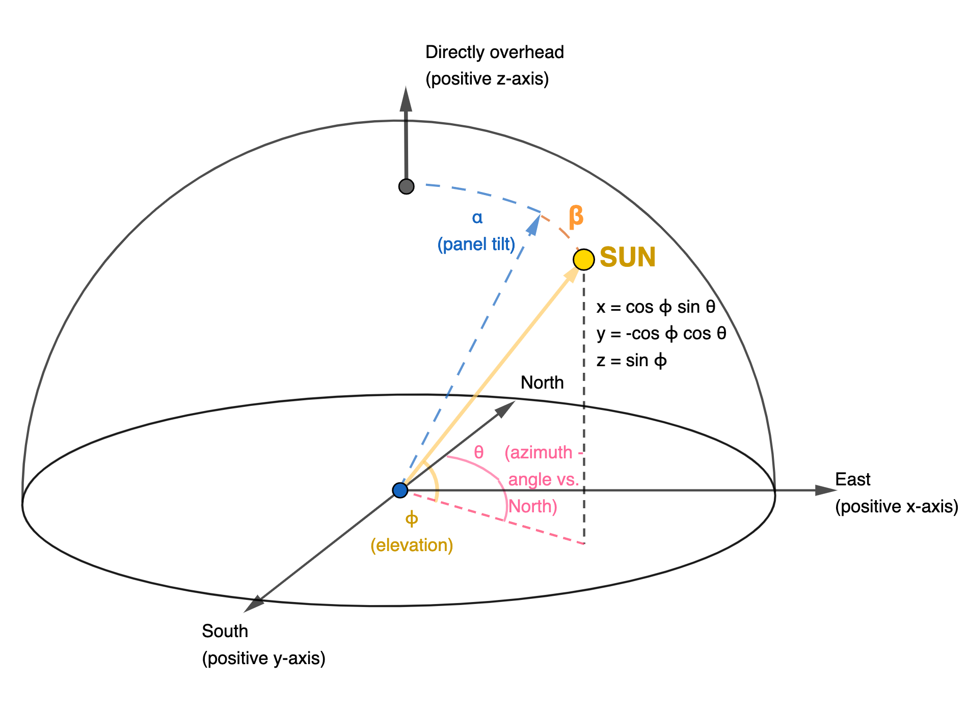
So we are looking for the angle, \(\beta\), between the dashed blue vector where the panel is pointing and the yellow vector representing the sun’s position. But our ultimate target is actually \(cos\ \beta\) to determine the solar flux onto the panel. Because the panel vector and the solar position vector are both unit vectors, \(cos\ \beta\) is simply the dot product of these two vectors. Hence:
\[cos\ \beta = sin\ \alpha\ cos\ \phi\ sin\ \theta + cos\ \alpha\ sin\ \phi\ \ \ \ (1)\]The solar operator only contols the tilt angle of the panels \(\alpha\). So to maximize solar power generation, I assume that the utility sets \(\alpha\) to maximize \(cos\ \beta\), i.e., we set \(\frac{\partial}{\partial{\alpha}}cos\ \beta = 0\). Taking the partial derivative of equation (1), we are looking to find \(\alpha\) such that:
\(0 = cos\ \alpha\ cos\ \phi\ sin\ \theta - sin\ \alpha\ sin\ \phi\).
Rearranging and dividing by \(cos\ \alpha\ sin\ \phi\) gets us that at the optimal tilt angle \(\alpha\),
\[tan\ \alpha\ = \frac{sin\ \theta}{tan\ \phi}\]For this article’s analysis, I don’t need the optimal \(\alpha\) itself. To estimate the solar output at different times of day, with different sun posiitons, I just need to solve for the value of \(\cos\ \beta\) at the optimal \(\alpha\). The expression for \(cos\ \beta\) uses both \(\cos\ \alpha\) and \(sin\ \alpha\), both of which can be derived from \(tan\ \alpha\):
\(cos\ \alpha\ = \dfrac{1}{\sqrt{1 + tan^2\ \alpha}} = \dfrac{tan\ \phi}{\sqrt{tan^2\ \phi + sin^2\ \theta}}\), and
\(sin\ \alpha\ = \dfrac{tan\ \alpha}{\sqrt{1 + tan^2\ \alpha}} = \dfrac{sin\ \theta}{\sqrt{tan^2\ \phi + sin^2\ \theta}}\).
These two expressions can now be substituted into the expression of \(cos\ \beta\) from equation (1):
\(cos\ \beta = \dfrac{sin^2\ \theta\ cos\ \phi}{\sqrt{tan^2\ \phi + sin^2\ \theta}} + \dfrac{tan\ \phi\ sin\ \phi}{\sqrt{tan^2\ \phi + sin^2\ \theta}}\), which ultimately simplifies to:
\[cos\ \beta = \sqrt{1 - cos^2\ \theta\ cos^2\ \phi}\]A quick gut check validates this formula: when the sun is due East or West, \(\theta\) is 90° or 270°, \(cos\ \theta\) is 0, so the entire expression simplifies to \(cos\ \beta = 1\). This makes sense because an East-West tilting panel can point straight at the sun and receive maximum solar flux. This is similarly true when the sun is directly overhead, with \(\phi =\) 90°, \(cos\ \phi = 0\) and \(cos\ \beta = 1\).
Adjusting for Lower Solar Intensity at Lower Angles
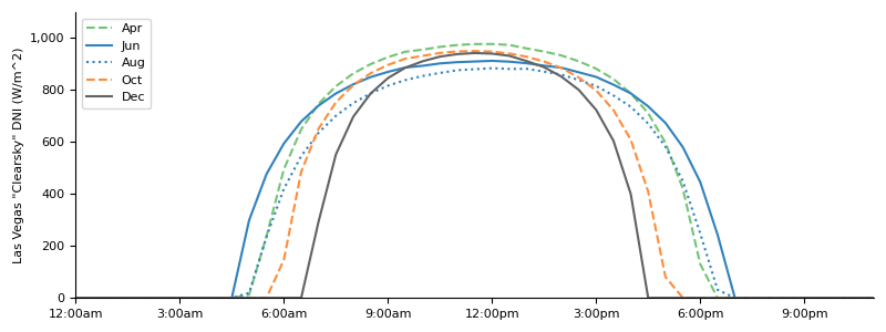
The last piece of this analysis is to reflect the fact that sunlight is less intense when the sun is lower in the sky – even with a panel pointed directly at the sun. This is because sunlight has to pass through more atmosphere (dimming it) at lower angles rather than higher angles. The intensity of the sunlight reaching a panel pointed directly at the sun (the panel surface is normal to the sunlight rays) is called Direct Normal Irradiance (“DNI”) and can be measured empirically at given locations.
The National Solar Radiation Database provides data sets of solar radiation metrics at various locations on the earth’s surface for every day in 10-minute increments. The chart below shows “Clearsky” DNI in Las Vegas from 2021, with all days in a given month averaged into a single time series (both to smooth out irregularities and to match my month-based analysis of generation data).
Putting It All Together
Finally, we can estimate total solar generation over the course of any day in Nevada by:
- Computing the solar angle positions \(\phi\) and \(\theta\) for the day and time at that location
- From those solar angles, determining the best angle to position a single-axis solar panel at to point most directly at the sun, and then what proportion of solar energy – i.e., \(cos\ \beta\) – can be captured at that angle
- Multiplying this proportion by the total direct solar radiation (DNI) reaching the ground at that time
The results of this exercise are shown below.
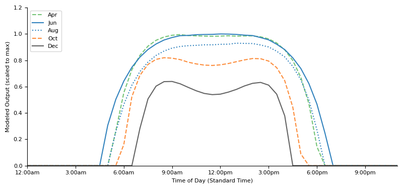
These modeled curves match the features of the actual solar generation curves shown up top, suggesting that my model of how utility solar panels work in Nevada is reasonably accurate.
(1) the extra long hours of near-peak generation throughout many hours of the day in summer that comes from being able to track the sun while it is high in the sky appears in the June curve above.
(2) The double-peak in winter months, with a trough in generation at mid-day when an east-west tilting panel cannot get as good an angle on the sun low in the sky in the south, as it can in the late morning / early afternoon when the sun, still low, is more east or west in the sky.
Other Features
The modeled outputs also captures the two less obvious features of the Nevada solar generation data described above.
First, April is indeeed better than August! Despite the solar angles (and the fraction of solar flux \(cos\ \beta\) that can get captured by panels) being similar between the two months, the intensity of sunlight in April is lower than in August. Whatever the atmospheric cause of this may be (temperature / humidity is higher in August), the higher spring than summer DNI levels directly follow through to electricity generation.
| Cos \(\beta\) April | Cos \(\beta\) August | DNI April | DNI August | |
|---|---|---|---|---|
| 8:00 a.m. | 0.98 | 0.99 | 860 | 747 |
| 12:00 noon | 0.89 | 0.93 | 973 | 862 |
| 4:00 p.m. | 0.99 | 0.99 | 784 | 733 |
Second, the winter months of December / January are particularly low-output. In other words, fall/spring output is closer to the higher summer levels than to the lower winter levels. This is a function of solar angles: from March through September there is always some time of day where the sun crosses the east-west axis and a single-axis panel can point directly at the sun. It is only in the winter months where this is not possible.
Shortcomings
The modeled analysis does diverge from observed data, including the fact that in the real world, winter output appears to be a higher proportion of summer output than in the modeled output. For example, the “real world” mid-day December level is about 70% of the mid-day June level, whereas in the modeled output this is about 55%.
The discrepancy could be from a number of sources, including:
- The fact that solar energy used for generation comes not from direct light of the sun (DNI) but also from diffuse light scattered from the entire sky; this component of light is less angle-sensitive
- Solar generation in Nevada may come from a number of different kinds of panels, not simply single-axis panels
- There could be “throttling” of generation, if the amount of power generated from solar panels exceeds either the power demanded at the time or transmission capabilities of the grid
Conclusion
Shortcomings notwithstanding, this exercise validates the premise that the physics of the world (the angle of the sun in the sky and how much radiation is absorbed by the atmosphere at different times of day) as well as engineering choices (how panel installations are built) predictably determine what is possible to expect from an energy generation installation.