Demand Pricing
In this post I return to the electricity pricing in the U.S., this time focusing on a concept that absent for most residential customers but mandatory for business customers that exceed a certain size: demand pricing. Under a demand pricing scheme, an electricity customer is charged in two separate ways:
(1) Consumption: Energy. Like residential plans, demand-based plans still charge for total energy consumption, measured in kilowatt-hours (kWh). The per-kWh charge may be fixed, may depend on the quantity used (i.e., more expensive as usage goes up) or it may depend on the season and time of day in a Time of Use plan.
(2) Demand: Power. In addition, utilities charge not just for energy consumed (in kWh) but also for the maximum rate of energy consumption in a short period of time (typically 15 or 30 minutes), at any time during the billing period (typically monthly). This is a measure of maximum power use rather than enregy consumption and so is priced on a per-kW basis. Demand charges can also depend on the season and time of day.
This post will discuss:
- Why the infrastructure costs and risks to grid stability from sharp fluctutations in power use by large customers justify demand-based pricing systems,
- How demand pricing creates different incentives for consumers than energy-consumption pricing alone, and how using electricity-consuming equipment in a staggered rather than parallel manner can meaningfully cut costs, and
- How different states structure their plans. In particular, different states have different ratios between energy consumption costs and demand costs, which leads to different strengths of economic incentives to smooth out energy usage over time.
Why is there a Demand Charge for Commercial and Industrial Customers?
The idea of pricing for peak demand (especially during heavy use periods such as summer afternoons) derives from the physical requirement that the grid continuously balance electricity supply and consumption. Large electricity consumers such as commercial and industrial users pose a greater risk to grid stability through sharp spikes in the quantity of electricity demanded – they may require bringing online additional “peaking” generation capacity and in the limit may result in more electricity being demanded than supplied. As such, usage spikes are priced at a premium, both to cover the infrastructure costs of the utility providing this flexibility as well as to incentivize a smoother usage profile by consumers.
National Grid, a utility operator in the northeast U.S., explains that while residential consumers have simple rate structures based on consumption because “there is relatively little variation in electricity use from home to home…”
This is not the case among commercial and industrial energy users, whose electricity use–both consumption and demand–vary greatly. Some need large amounts of electricity once in a while–others, almost constantly. Complicating this is the fact that electricity cannot be stored. It must be generated and supplied to each customer as it is called for–instantly, day or night, in extremely variable quantities. Meeting these customers’ needs requires keeping a vast array of expensive equipment–transformers, wires, substations and even generating stations–on constant standby. The amount and size of this equipment must be large enough to meet peak consumption periods, i.e., when the need for electricity is highest.1
A Gentle Introduction to Demand
A Simple Pricing Plan (Nevada)
We’ll begin with a simple example: the Southern Nevada LGS-1 plan, which is for medium sized businesses (monthly consumption averaging above 3,500 kWh2 and demand < 200 kWh), and is constant throughout times of day and seasons. There is also a time-of-use plan available (described below).
This plan has an $0.114 / kWh usage charge, and $7.69 demand charge. Note that the demand charge is quoted in dollars per kW rather than the usage charge in cents per kWh, indicating that a business’s energy bill is more sensitive to how much its electricity usage peaks at its maximum consumption point in a month, than to its overall usage.
A medical facility that uses 8,000 kWh per month but is open only 20 days a month for 10 hours and high air conditioning use during those hours, might have an average usage of 40 kW but a peak demand of 100 kW, and thus be charged $8,000 kWh \times $0.114 / kWh + 100 kW \times $7.69 / kW = $1,681.$
Meanwhile a small highly automated manufacturing facility with limited human staffing and HVAC use may have its machines running 25 days a month for 16 hours, of an average usage of 20 kW but with a peak demand of only 40 kW. Its charge will be $8,000 kWh \times $0.114 + 40 kW \times $7.69 / kW = $1,220.$ The automated facility has a 25% lower energy bill with the same usage, solely because its use is more spread out and has a lower peak power consumption than the HVAC-intensive medical facility.
An Example from Real Life
Ignoring the fact that I am a residential customer, two days of my home’s electricity consumption in August 2022, shown below, illustrate the impact of demand vs. energy consumption pricing. August 16, 2022 was a hot summer day in Southern Nevada, and it is easy to see the operation in the afternoon and early evening of my two central air-conditiong units, each of which can consume ~1 kWh in 15-minute increments (~4 kW power). Note that the highest consumption was around 5pm, with both A/C units running and using a total of 3.5 kWh in 15 minutes, which is an average demand power of ~14 kW during this period.
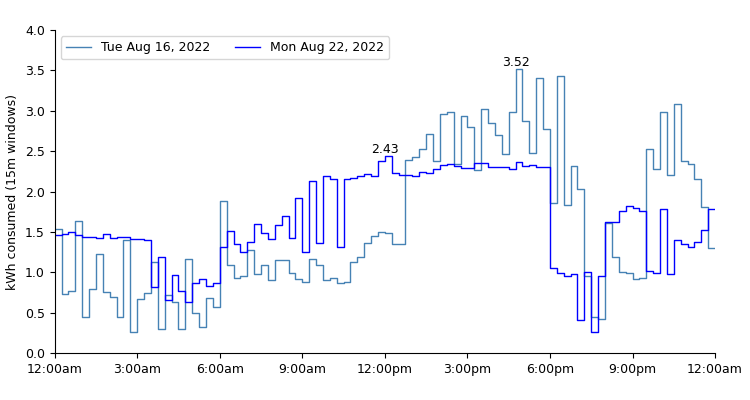
August 22 was similarly a hot day, but I had only one operational A/C because the second was waiting for repairs. The single unit struggled to cool the house during the hottest part of the day, and made up for that by operating many more hours (like the automated manufacturer in the above example). The highest 15-minute period of consumption was 2.4 kWh around noon (probably the A/C plus the oven working on lunch), a demand of ~9.6 kW.
The total consumption on these days was similar, with the one-A/C day using slightly more total energy (155.9 kWh vs. 150.2). So under a residential billing program based on energy consumption, the two-A/C set-up would be cheaper. But because it had a higher maximum power draw, the demand charge inverts the cost, making the two A/C unit more expensive assuming a 30-day month of identical days. Details below:
| Day’s Usage (kWh) | Monthly Usage (kWh) | Peak Demand (kW) | Usage Cost | Demand Cost | Total Cost | |
|---|---|---|---|---|---|---|
| 1 A/C Unit | 155.9 | 4,676 | 9.7 | $533.03 | $74.89 | $607.90 |
| 2 A/C Units | 150.2 | 4,504 | 14.1 | $513.41 | $108.18 | $621.59 |
This example is contrived: my house was much more unpleasant with a single A/C unit than with two: the zone with the working unit was too cold and the side with the broken unit was too hot. But it illustrates the point that demand (power) vs. usage (energy) may cause price incentives to point in different directions.
Staggered vs. Parallel Use of Equipment
A second real-world example depicts the electricity usage over 6 days of San Diego-based friends with an electric vehicle. Visible in the chart is the overnight EV charging at 8 kW of power (it is scheduled to end at 6:00 am, and begins however long is needed before that to fully charge the car), as well as the running of their pool filter at about 1.5 kW from 5:00 to 11:00 am.
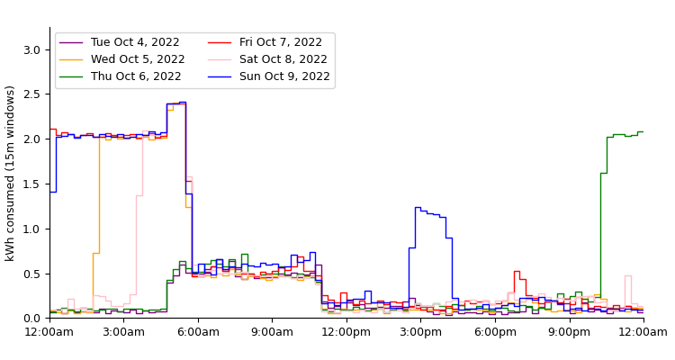
The overlap of EV charging and pool filter between 5 and 6am is the time of their peak demand. The overlap causes the energy consumption during this hour to be about 0.4 kWh higher in each 15 minute period. Shifting the pool filter’s run time an hour later would leave total energy consumption exactly the same (about 40 kWh per day). But eliminating the overlap would reduce peak demand during this period by 1.3 kW from 9.64 kW to 8.34 kW. In the Nevada fixed-rate plan described above, this would save about $10 per month. Under San Diego commercial plans, in which demand is priced at $60 / kW, this would save $80 per month.3
For actual commercial and industrial users, with electricity usage hundreds or thousands the magnitudes described here, managing the operation of power-hungry equipment to be sequential rather than parallel can generate large cost reductions (and downstream grid stability benefits).
Rate Structures in Different States
Simple Structures
The table below presents a few examples of demand-based business rates in different U.S. states. Often, a customer ends up in a rate category based on their usage patterns.
| Nevada (NV Energy) | Florida (FPL) | Virginia (Dominion) | |||||
|---|---|---|---|---|---|---|---|
| Plan Name | LGS-1 | OLGS-1 | General Service Demand | Gen. Svc. Demand-TOU | Small General (5P) | Large General (6P) | |
| Applicable customers: | Medium (monthly usage > 3500 kWh, demand < 200 kW) | All businesses other than small businesses | Demand < 500 kW | Demand > 500 kW | |||
| Time-of-Use? | No | Yes | No | Yes | Yes | Yes | |
| Summer Peak | Energy / kWh | $0.114 | $0.209 | $0.068 | $0.100 | $0.056 | $0.041 |
| Demand / kW | $7.69 | $11.28 | $11.29 | $11.29 | $11.77 | $15.33 | |
| Summer Off-Peak | Energy / kWh | Same | $0.106 | Same | $0.055 | $0.040 | $0.035 |
| Demand / kW | $0.00 | $0.00 | $0.00 | $0.00 | |||
| Winter Peak | Energy / kWh | $0.105 | $0.100 | $0.056 | Same as summer | ||
| Demand / kW | $3.97 | $11.29 | $9.21 | ||||
| Winter Off-Peak | Energy / kWh | Winter has 1 rate only |
$0.055 | $0.040 | |||
| Demand / kW | $0.00 | $0.00 | |||||
A couple of points to notice:
Off-Peak Demand Doesn’t Matter Much. Pricing plans that charge more for energy usage during peak times (e.g., summer afternoons) apply the same idea to demand charges as well. In fact, the differential in demand pricing is more stark: both Nevada and Florida plans listed above have non-zero demand charges only for peak periods (Nevada has no peak/off-peak distinction in winter): the maximum power consumption during off-peak hours is totally ignored.
This set-up suggests that it is system-wide constraints, such as finite generation capacity, that demand pricing is primarily targeting, since that constraint is tested only during peak system-wide usage periods. The costs of stressing more local constraints such as local transmission and transformer equipment are more applcable at all times, and would justify higher demand charges during off-peak hours than we see here.
Demand vs. Consumption Exchange Ratio. Recall that power demand is priced in dollars (per kW) whereas energy consumption is priced in cents (per kWh). This means that an extra kWh consumed at the moment of peak demand costs multiples of a kWh consumed at any other time.
For example, in Nevada’s TOU plan, an extra kWh of consumption during the peak hour of the month costs $11.28 during the summer. At any other peak time it costs 21 cents. The cost of incremental demand is thus 54x that of the cost of incremental consumption. Florida and Virginia’s ratios are 113x and 374x. A more complicated San Diego plan has a ~$60 / kW demand charge with incremental consumption almost free: $0.023 / kWh, a 2600x ratio.
The differences in these exchange ratios may rationally reflect differential marginal costs of the grid supplying incremental peak electricity vs. non-peak electricity. A moderate ratio between demand and consumption charges may (like the cost difference between peak and off-peak consumption) simply reflect higher fuel costs at peak times. Solar may make the incremental kWh nearly free at noon, but the need to use coal or natural gas during the most likely peak hours means higher fuel costs.
A high ratio as in San Diego may reflect one of two things. First, California is awash with solar-generated kWh during the middle of the day, but still experiences a large ramp-up in power demanded in the early evening. This means incremental demand during peak periods is particularly risky to grid stability, justifying a much higher price than incremental consumption at other times. Second, it may mean that peak consumption does not only require more fuel to be spent but may be testing the limits of generation capacity available: the marginal cost may actually reflect the high capital costs of building additional peaking generation capacity.
Economic costs may not be the only driver of these differences, however. The setting of electric rates – typically requiring state public utility commission approval – is a political process and therefore may reflect the policy preferences of non-economic stakeholders as well.
Energy Price as a Function of Smoothness
Another way to think about the two dimensions of price (demand and energy consumption) is that the plans offer a variable price per kWh of energy consumed, as a function of how evenly that energy consumption is spread throughout the billign period.
Returning to the air conditioning example: with 2 A/C units, my peak demand was 14.1 kW. The total daily energy usage – 150.2 kWh – was the equivalent of 10.7 hours of peak power. With 1 A/C, my peak demand was 9.7 kW. The total daily energy usage (155.9 kWh) was the equivalent of 16.1 hours at peak power.
Taking the total costs (demand plus energy charges) and dividing by the quantity of energy consumed, we get a blended cost per kWh. That number is lower for the more constant consumption (more hours per day) than for the more jagged consumption running fewer hours per day.
| Day’s Usage (kWh) | Peak Demand (kW) | Equivalent Hours / Day | Monthly kWh | Monthly Cost | Blended Cost per kWh | |
|---|---|---|---|---|---|---|
| 1 A/C Unit | 155.9 | 9.7 | 16.1 | 4,676 | $607.90 | $0.130 |
| 2 A/C Units | 150.2 | 14.1 | 10.7 | 4,504 | $621.59 | $0.138 |
It’s bit counterintuitive that a much smoother consumption profile (16.1 hours vs. 10.7 hours) produces only a 6% decrease in the per-kWh cost of electricity. But this is a function of the low 54x ratio in the Nevada non-TOU plan between the demand charge and energy consumption charge. The graph below plots the blended cost per kWh as a function of hours per day active, for three state plans listed above (Nevada, Florida, Virginia):
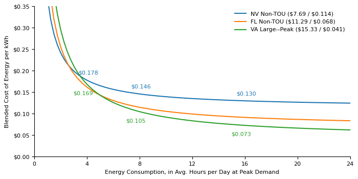
In the Virginia plan, with its 374x ratio of demand to consumption charges, there is a much higher incentive to smoothe out the energy profile: the 2 A/C profile at 10.7 hours / day costs 8.9 cents per kWh whereas the 1 A/C profile at 16.1 hours per day costs 7.3 cents per kWh, an 18% decrease.
Commercial-scale Thought Experiment
Imagine a global sreaming-video service whose customers watch videos between 7:00pm and 11:00pm local time. It may choose to have a data center in each geographical region so that video data sits geographically close to customers in that region and thus has low latency. With this strategy, each data center may only operate near peak power consumption around 4 hours each day (7 to 11pm).
If latency is not a major concern (perhaps users’ devices can buffer 1-2 minutes of video), the company may consolidate into only a few large data centers that run nearly all the time. 7 to 11pm in many global time zones may mean data centers are running near peak power consumption 16 hours per day.
Clearly these choices have different capital costs, but for a large commercial electricity user with data centers, energy costs will also be material. Under a plan like Virginia’s with high demand costs relative to energy costs, consolidating into fewer data centers that run 16 hours a day instead of 4 hours at peak power would lower energy costs by more than 50% (e.g., from $0.169 to $0.073 per kWh).4
Further Work
This post has introduced the mechanics of simple demand pricing plans, the economic rationale for them on the supply side, and how consumers can think about them on the demand side.
The next post will dive into more variants of demand pricing, in which demand-based pricing can be based on inputs more varied than a simple measure of “this month’s maximum power.”
-
FPL uses a water delivery analogy. While most customers can be served with a standard one-inch-pipe, one who uses significant water in bursts will require special equipment from the water company (larger main lines or service pipes), with “demand” charges covering the costs of equipment needed to handle more flow than standard. ↩
-
Business customers below this threshold are charged for energy consumption only, like residential customers. ↩
-
In the real world, since these are residential customers they are not charged for demand. Instead, they would save money by running their pool filter between midnight and 6am as well, which are super-off peak hours with energy charges of ~$0.15 instead of ~$0.45 per kWH. ↩
-
In a similar vein, always-on data centers like the type used by cryptocurrency miners have a particularly synergistic relationship with baseload power operators like nuclear power plants. The generator benefits from having a consistent demand without fluctuation from other grid users, and the consumer can thereby receive lower energy prices. ↩